
Introduction
Finite Element Analysis of Vehicles and Tires has become a very important aspect of tire design and failure analysis for most Tire companies. Tire modeling with ABAQUS is a very complicated process involving complex materials like hyperelastic rubber and textile reinforcements, large model sizes, prolonged simulation time, and various convergence issues. This white paper intends to help in understanding the challenges in tire analysis and several tips and tricks that make a difference in the quality of the results and processing time. AEG hopes that this article, which covers the challenges of tire design optimization using ABAQUS and includes footprint analysis, will be useful to ABAQUS users in this field.
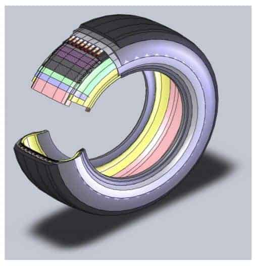
A general tire has the following major tire components
- Tread
- Belt Region
- Inner Liner
- Sidewall Region
- Inner Carcass Region
- Bead Filler Region
- Apex/Chafer Region
- Beads
- Reinforcements
- Nylon Cap Ply
- Steel BeltsCarcass Ply
Constructing the structure of the tire and modeling each component is the first step in the analysis. AEG found that utilizing the combination of AutoCAD and ABAQUS-Sketch is a very good way to start the modeling. It is important to have the understanding that when an AutoCAD drawing is imported to ABAQUS sketch it creates splines and contains a large number of node points. A thorough simplification of the geometry is recommended, i.e. flattening up crooked lines, reducing the number of nodes, deleting unnecessary wedges or fringes, taking off rounds/fillets, and simplifying the corners is highly recommended. In this process, the dimension and shape and the tire should not be compromised. If the geometric complexities can be avoided at this point, it will save a considerable amount of computational time, money, and resources later.
Features in the sketch module of ABAQUS such as offset can be intelligently used to maintain excellent dimensioning consistency of the different reinforcement layers inside the tire. ABAQUS has a very comprehensive guideline for tire analysis in their example manual and it has been proved that an axisymmetric modeling approach with half geometry is the best way to start the modeling. Also, it is widely accepted by the FEA community in the Tire industry that a smooth tire model (3D model by revolving a 2D tire model by 360°) is insufficient enough to capture the overall efficiency of the core design. The complex tread geometry with random pitch or asymmetry in the thread can be used in the later stages to get very accurate results for a specific tire design model. The basic steps for tire FEA analysis can be described below.
- 2D axisymmetric Tire geometry modeling
- 2D Rim Mounting and Inflation Analysis
- 3D model generation by Revolve and Reflect features in Symmetric ModelGeneration (SMG) option in ABAQUS
- Footprint Analysis with rated load and rated inflation pressure
- Steady state rolling analysis using Steady State Transport option in ABAQUS
- Dynamic Analysis, Hydroplaning analysis
2D Axisymmetric Tire Model Design
AEG recommends the following guidelines to model the 2D axisymmetric analysis for tire design.
- The lip or fringes on the sidewall is not a necessary feature for tire analysis but it becomes a burden as it increases the number of elements during meshing. So deactivating the features is a good idea.
- Instead of modeling the cluster of strands of small diameter wires hosted inside the rubber, the bead can be modeled with a single cross-sectional area. The area should match the total cross-section area of the bead region. Now as this bead constitutes steel wires embedded in the rubber, Young’s modulus of the steel can not be used as the material. Young’s modulus should be modified on the basis of the ratio of the total steel wire cross-section area to the total bead region area. An approximation of half of Young’s modulus of steel can be a good starting point.
- The curvature of the tread surface and the tread shoulder plays a significant amount of role in the footprint analysis, so getting the curvatures right is very important.
- All the different regions can be modeled as different parts initially, but it is important to assemble them and create a single part with different regions by performing a merge operation in the assembly module. This ensures that there is a single part of the core containing no gap between the regions and also the complexities of interaction or tie constraints can be avoided in this way. The reinforcement can be modeled separately as parts and embedded inside the host regions in the assembly module later.
- The reinforcements like nylon caps, steel belts, and Carcass plies need to be drawn with precision and special attention should be given to the dimensions of the following features.
- the width or span of the reinforcements
- the gap between different reinforcements
- the continuity of the lines
The offset feature of ABAQUS Sketch was found to be very useful for this purpose.
- The reinforcements can be modeled as rebar layers which allow users to specify the cross-section area of the strands, the gap between two strands, and the alignment angles of the threads. In real the strands comprise multiple thin threads but during modeling, it is safe to combine all the threads and use a single-cross section area for the strand. A micro-modeling concept can be used if the detailed effect of the threads on the analysis is required. Abaqus lets the users use an option called lift equation parameters that takes care of some amount of pre-stress which accumulates during the time of curing.
- The reinforcements can be meshed with either membrane elements or surface elements. Both elements have rebar options associated with them. The membrane element is advantageous sometimes as the inter-laminar shear stress (S12) inside the rebar layer can be obtained as an output in the post-processor. Membrane elements also offer an option of providing a thickness of the rebar which can lead to some inaccuracy in the results as the rebar host material and the embedding host material superimpose each other. Though the surface element does not produce any stress output, it is a safer way of modeling as it does not have any material superimposition effect and the complexities associated with it.
- It is important to understand that this tire model can be meshed with lower order tetrahedral elements. Abaqus analysts have tried and tested the lower order tetrahedral elements and found that they provide pretty accurate results. This actually saves a lot of time that would have been wasted in meshing the tire regions with structural quadrilateral elements. A generous number of elements are needed (for example 1000) when meshing the 2D axisymmetric model with tetrahedral elements. Both the axis-symmetric quadrilateral and axis-symmetric triangular elements with a twist, CGAX4, and CGAX3 are suitable for meshing. Interestingly it should be noted that these are full-order elements and also they are not reduced order, using these elements can give much faster convergence and accurate results.
- A debate can arise on what type of element is suitable for tire analysis. AnABAQUS tutorial recommends using hybrid elements for any hyperelastic material problem. Hybrid elements are incompressible elements with Poisson’sratio very close to 5. But when it undergoes large compressive stress in the area under the belt regions it sometimes forces the solver to march very slowly thus creating convergence problems. Also, the hybrid elements have been observed to work well in the 2D model but fail in the 3D model. To bypass this problem it is recommended not to use a hybrid material, instead, it is advisable to use a general full order element (not reduced order element) with Poisson’s ratio of 0.495 or very close to but less than 5. For Neo Hookian model and Mooney Rivlin model, the value of D1 can be calculated using this Poisson’s ratio by the following equation
D1 = 3(1 – 2v) / G(1 + v) where G = 2(C10 + C01)
G = Shear Modulus
V = Poisson’s ratio
- The material property selection of the Nylon and Textile material for the carcass ply is very important. A Marlow model can be used for the material instead of using only Young’s modulus if test data is available for these materials.
- For modeling the hyperelastic rubber it is best advised to use Mooney-Rivlincoefficients. For modeling the hard and elastic rubber, Young’s modulus might not be sufficient and a Neo-Hookian model would be a better approximation.
- All the regions and the reinforcements need to be saved as sets for post-processing of the data.
- The foot region of the tread needs to be saved as set for future use in 3D footprint analysis.
- From first-hand experience, we can claim that all these suggested changes make a huge impact on the solver’s time and convergence in tire design.
2D Rim Mounting and Inflation Analysis
- The rim can be modeled using an analytical rigid surface. The contact surface needs to be defined in advance. A reference point should be placed in a strategic location.
- The two main boundary conditions are the fixing of the rim in all d.o.f and providing a symmetric boundary condition on the symmetric line of the model. The rim width can easily be changed by displacing the rim before any analysis.
- The contact interaction between the rim and the tire toe can be defined in various ways.
- To get a quick result without actually designing the rim it is possible to fix some node points on the toe of the tire and simulate the effect of hard contact of the tire on the rim. This will not allow the tire to slip on the rim but would provide a quick result by avoiding contact interaction which is time-consuming.
- Instead of the whole rim geometry a small analytical rim curve can be drawn and after associating with a reference point it can be used as the rim.
- The full rim geometry can be modeled and imported for analysis.
- It is also very helpful if the inflation analysis is done in two steps. In the first step, a small amount of surface pressure can be used to initiate contact between the tire and the rim and then in the second step, the full rated pressure can be applied. These tactics save the solver from unnecessary cutbacks and convergence problems.
- Contact interaction with a friction coefficient of less than 0.2 is highly recommended for a very easy convergence. When the friction coefficient is greater than 0.2 the solver automatically chooses unsymmetric matrix storage, which gives out accurate results but has convergence problems and long run time associated with it. Also if it is really needed to use a larger coefficient of friction it can be used in the second step of the analysis.
- The main load is the pressure applied to the inside surface of the 2D model and the tire.
- ABAQUS models don’t have units associated with them so the units of dimension, material properties, and loads should be consistent all along the tire design.
- When running this analysis the Abaqus environment file needs to be modified and the following lines need to be definitely added to the environment file.
- pre_memory = “2048mb” number depends on the computer ram sizestandard_memory=”2048mb” cae_no_parts_input_file=ON Max_history_requests=0
The second option flattens the inp file and only writes necessary features which helps in producing appropriate *.res files, The *.res file can be obtained when the restart request field is set to non-zero frequency values.
3D Tire model generation by Revolve and Reflect features
After the rim mounting and inflation analysis are complete, the 2D half tire model can be revolved using the Symmetric model generation option in ABAQUS and a 3D model can be created. A separate analytical Surface can be created as a road model and pressed against the tire to get a footprint of the tire. The main results that interest the designer are the average contact pressure, maximum contact pressure, the contact pressure distribution, shape of the footprint area, total area, contact area, and also the void area of the footprint.
- The model is first revolved, footprint analysis is performed and then the model is reflected to get the full picture of the 3D tire design. It is interesting to note that the sequence here is important as the reflected feature cannot be used on 2D elements.
- The footprint analysis on the 3D model is a critical analysis involving coding in the inp files as the SMG option is not supported by the ABAQUS CAE. Each line of the inp file is important and requires proper understanding. When running the codes ABAQUS command prompt needs to be used and previous result files(*.res) are needed for result transfer.
- ABAQUS has developed cylindrical elements, including those for the tire industry, which can be used for 3D modeling and foot print analysis. The footprint region needs to be general elements and the remaining section can be modeled with cylindrical elements. It is advisable to use a gradient approach in the cylindrical element set up so that there remains continuity in the full model. These elements contain mid-nodes, but overall behave like a poly element and are claimed to be successful in providing accurate results.
- To facilitate the contact between the tire and the road, an element set in the footprint regions should be created in the inp files by utilizing the node numbers on the surface of the Tread. Also, the symmetric equation in 3D should be substituted by symmetric equations during footprint analysis.
Foot Print Analysis of tire design with rated load and rated inflation pressure
- The inflation results can be transferred to the 3D tire model from the 2D model and brought into equilibrium using a dummy step. Though the dummy step transfers results it should be properly defined with the step definitions, boundary conditions, and the inflation pressure as the load.
- The footprint analysis can be divided into two more steps.
- displacement controlled loading and
- Load controlled loading.
It is favorable if the contact between the road and the tread surface is established before the actual load is applied, so in displacement-controlled loading, the road is moved by a know distance such that it comes in contact with the tread surface. The friction coefficient should be kept less than 0.2 and the initial value of the time step adjusted for better convergence.
- In the next step, the actual load should be applied. As this is a half model, the rated load that should be used here is half of the actual rated load. Some tricks that affect the solution procedure are noted below.
- It was noted that if the boundary conditions were defined afresh in each step the solver converges much faster.
- A lower friction coefficient (<2.0) always helps in convergence though higher values can be used in this step if needed.
- default slip tolerance of 0.5% can be used in each case of friction definition.
- Separate contact control with stabilize option can be defined to stabilize the contact between the tire and the rim.
- To obtain accurate stress values and footprint area, it’s crucial to define CAREA, CFN, and CPRESS in the History output field during foot print analysis.
- The results obtained can be post-processed in ABAQUS using the mirror option in the Viewer to get the images of a full tire design model.
Steady State Rolling analysis using Steady State Transport option
- After the footprint analysis, for the steady state rolling analysis, a full model is needed so the half-footprint model should be reflected and the full model created.
- In the steady state analysis, the contact problem between the rim and the tire can be avoided by specifying a set of nodes on the tire toe as fixed nodes. This would save considerable simulation time and also save from tough convergence issues. When applying the boundary conditions on the node sets, it is advisable to utilize the kinematic coupling option on all the d.o.f of these nodes.
- The steps that a steady-state rolling analysis should follow are given below.
- Datacheck the 2D axis model
- Data check the half 3D model by using SMG revolve option using the previous output result file.
- Data check the full 3D model by using SMG reflect option using the previous output result filed.
- Perform all the steps, inflation, displacement-controlled loading, and load-controlled loading.
- The steady-state transport analysis should run now.
- The slip angle change can be performed now
Steady State Rolling Analysis – The Steady-state transport option needs to be used here along with the *TRANSPORT VELOCITY option to specify the angular velocity of the tire and *MOTION, TYPE=VELOCITY, TRANSLATION option to specify the linear velocity of the tire. This option works on Node sets, so the entire tire model is saved as NTIRE in this program.
- There are two distinct analysis in SSR
- Braking Analysis – Smaller angular velocity should be used here. The angular velocity can be calculated by using the deformed radius and the linear velocity of the tire.
- Traction Analysis – Higher angular velocity should be used here. The angular velocity can be calculated from the undeformed radius and the linear velocity of the tire.
The angular velocity calculations need not be precise because, in the end, we would be looking forward to finding out the free-rolling velocity. When the force or torque on the spindle is observed, it can be found that the force and torque pass through the zero value and change sign when the phase changes from braking to traction. The angular velocity corresponding to zero torque is termed as free rolling velocity and the state is known as free rolling equilibrium state.
The rolling analysis gives a decent demonstration of how the tire design would perform when it is moving and provides valuable information on different stress/strain energy density values that can measure the dynamic efficiency of the tire.
Santanu Chandra, PhD
Project Engineer, American Engineering Group